[MITx: 6.00.1x] Introduction to Computer Science and Programming Using Python (Week 7) – Simple Plot

สำหรับ Blog อันนี้เป็น Lecture สุดท้ายสำหรับในการเรียน หลังจากการเรียนที่ผมเขียนไปใน Blog ตอนที่แล้ว ในตอนนี้เรานำข้อมูลมาแสดงให้เห็นภาพ (Visualize) โดยนำข้อมูลมา Plot เป็นกราฟ โดยใช้ Library ตัว PyLab ครับ สำหรับการใช้เรานั้น เราต้อง import ข้อมูลก่อนครับ โดยใช้คำสั่ง ดังนี้

import pylab as plt
# เวลาใช้งาน ใช้ plt.<ชื่อ Method ได้เลย>

ลองกำหนด Sample Data กัน

📊 การกำหนด Sample Data ใน Class นี้ คุณ Eric Grimson พยายามเชื่อมโยงไปถึงบทที่แล้วครับ โดยใข้ Code ดังนี้

mySamples = []
myLinear = []
myQuadratic = []
myCubic = []
myExponential = []

for i in range(0, 30):
    mySamples.append(i)
    myLinear.append(i)
    myQuadratic.append(i**2)
    myCubic.append(i**3)
    myExponential.append(1.5**i)

Plot Graph กันเถอะ

📊 Version แรกครับ ใช้ Code แบบ Simple เลยครับ เอาให้มี Graph ขึ้นมาก่อนครับ โดยใช้ Code ดังนี้

plt.plot(mySamples, myLinear)
plt.plot(mySamples, myQuadratic)
plt.plot(mySamples, myCubic)
plt.plot(mySamples, myExponential)

📊 ผลลัพธ์ที่ได้

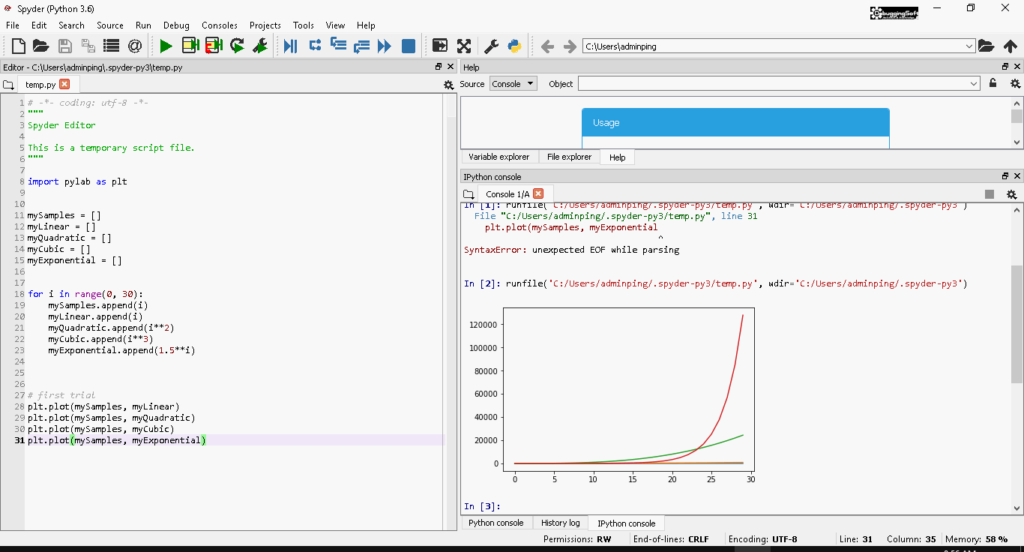
📊 จาก Version แรก พบปัญหา ดังนี้

• Plot ของตัว Linear กับ Quadratic มันมองไม่เห็นเลยครับ เส้นมันทับกัน - ต้องมาปรับ Scale ใช้ตัว xlim กับ ylim มาช่วยก่อนทำการ Plot ครับ

# Note
# plt.xlim(start,end)
# plt.ylim(start,end)

# Example
plt.ylim(0,1000)
plt.plot(mySamples, myLinear)

• ไม่รู้ว่าเส้นไหน เป็นการแสดงผลของข้อมูลอะไร - ใช้ Legend มาช่วย โดยเอาข้อมูลจาก Function Plot ตามที่ Highlight ได้ มาแสดงผลครับ

• ยังขาดพวก Title - เติม title ดิ

plt.title('Computational complexity of an algorithm')

• ยังขาดพวก ข้อมูลที่บอกว่าแกน x แกน y ว่าเป็นการแสดงข้อมูลอะไรครับ - ใช้ Label ช่วย เช่น

plt.xlabel('sample points')
plt.ylabel('linear function')

• ลองมาดู Code รวมๆ กันครับ

plt.xlabel('sample points')
plt.ylabel('Order of growth')
plt.ylim(0, 14000)
plt.plot(mySamples, myLinear, label = 'Linear', linewidth = 2.0)
plt.plot(mySamples, myQuadratic, label = 'Quadratic', linewidth = 2.0)
plt.plot(mySamples, myCubic, label = 'cubic', linewidth = 2.0)
plt.plot(mySamples, myExponential, label = 'Exponential', linewidth = 2.0)
plt.legend()
plt.title('Computational complexity of an algorithm')

📊 มาดูผลลัพธ์ที่ปรับกันครับ

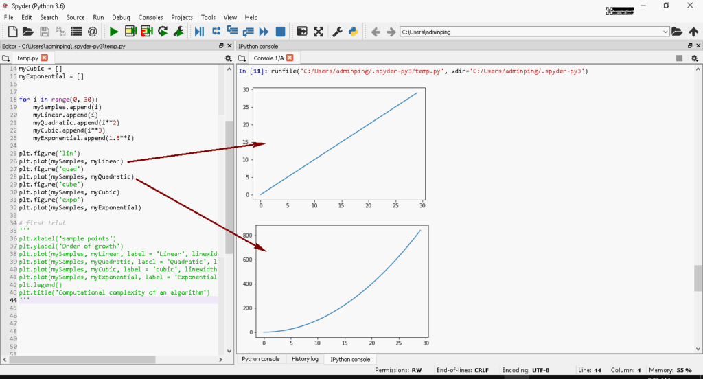
📶 ข้อสังเกตุ 1: อยากแยก กราฟออกจากกัน ใช้ Figure ช่วยได้

• Code ที่ทดสอบมี ดังนี้

plt.figure('lin')
plt.plot(mySamples, myLinear)
plt.figure('quad')
plt.plot(mySamples, myQuadratic)
plt.figure('cube')
plt.plot(mySamples, myCubic)
plt.figure('expo')
plt.plot(mySamples, myExponential)

• ลองดูผลลัพธ์ที่ได้ ผมได้ลากลูกศรประกอบไว้ แล้ว แต่พื้นที่มันน้อยเลยไม่สามารถ Capture มาได้ทุกแบบครับ

📶 ข้อสังเกตุ 2: ปัญหา ใน Method Plot แรก คือ การกำหนดพื้นที่การเขียนครับ จาก Code ตัวอย่างคือ mySamples ตัว PyLab มันจองยาวจนกว่าจะปิดโปรแกรมครับ ถ้าอ้างอิงไม่ดีข้อมูลมาเขียนทับกันครับ ซึ่งสามารถแก้ไขแก้ไข โดยใช้คำสั่ง Clear ก่อน Plot ครับ

plt.clf()
# plot something
plt.plot(mySamples, myLinear)

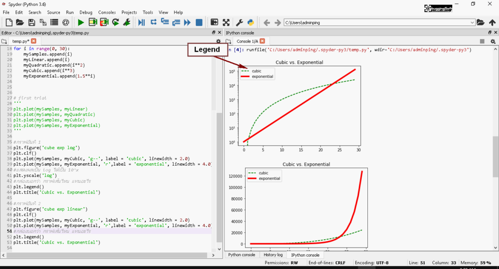
📶 ลองทำแบบอื่นๆบ้าง ตาม Code โดยคำอธิบายอยู่ใน Code ครับ

# ข้อมูลจากอันแรก
# กราฟอันที่ 1
plt.figure('cube exp log')
plt.clf()
plt.plot(mySamples, myCubic, 'g--', label = 'cubic', linewidth = 2.0)
plt.plot(mySamples, myExponential, 'r',label = 'exponential', linewidth = 4.0)
# แสดงผลเป็น log ได้เป็น 10^x
plt.yscale('log')
# กล่องบอกว่า กราฟเส้นไหน แทนอะไร
plt.legend()
plt.title('Cubic vs. Exponential')

# กราฟอันที่ 2
plt.figure('cube exp linear')
plt.clf()
plt.plot(mySamples, myCubic, 'g--', label = 'cubic', linewidth = 2.0)
plt.plot(mySamples, myExponential, 'r',label = 'exponential', linewidth = 4.0)
# กล่องบอกว่า กราฟเส้นไหน แทนอะไร
plt.legend()
plt.title('Cubic vs. Exponential')

📶 ผลลัพธ์ที่ได้

สำหรับบทนี้ ผมต้องกลับมาใช้ตัว Anaconda ครับ ตัว repl.it ไม่ Support การแสดงผลของ Library PyLab ครับ อดไปเล่นผ่าน Tablet เลยยย และส่วนเนื้อหา ถ้าอยากรู้เพิ่มเติม ทางผู้สอนบอกว่ามีสอนใน Course [MITx: 6.00.2x] ครับ

Reference

• PyLab Example - http://matplotlib.org/2.0.1/examples/pylab_examples/index.html